Teaching Simpson’s paradox at elementary school

Robert Siegler participates in the “Center for Improved Learning of Fractions” (CILF) and was chair of the IES 2010 research group “Developing Effective Fractions Instruction for Kindergarten Through 8th Grade” (report) (video).

IES 2010 key advice number 3 is:

“Help students understand why procedures for computations with fractions make sense.”

The first example of this helping to understand is:

“A common mistake students make when faced with fractions that have unlike denominators is to add both numerators and denominators. [ref 88] Certain representa­tions can provide visual cues to help students see the need for common denominators.” (Siegler et al. (2010:32), refering to Cramer, K., & Wyberg, T. (2009))

For a / b “and” c / d kids are supposed to find (ad + bc) / (bd) instead of (a + c) / (b + d).

Obviously this is a matter of definition. For “plus” we define: a / b + c / d = (ad + bc) / (bd).

But we can also define “superplus”: a / b ⊕ c / d =  (a + c) / (b + d).

The crux lies in “and” that might not always be “plus”.

When (a + c) / (b + d) makes sense

There are cases where (a + c) / (b + d) makes eminent sense. For example, when a / b is the batting average in the Fall-Winter season and c / d the batting average in the Spring-Summer season, then the annual (weighted) batting average is exactly (a + c) / (b + d). Kids would calculate correctly, and Siegler et al. (2010) are suggesting that the kids would make a wrong calculation ?

The “superplus” outcome is called the “mediant“. See a Wolfram Demonstrations project case with batting scores.

Adding up fractions of the same pizza thus differs from averaging over more pizzas.

We thus observe:

• Kids live in a world in which (a + c) / (b + d) makes eminent sense.
• Telling them that this is “a mistaken calculation” is actually quite confusing for them.
• Thus it is better teaching practice to explain to them when it makes sense.

There is no alternative but to explain Simpson’s paradox also in elementary school. See the discussion about the paradox in the former weblog entry. The issue for today is how to translate this to elementary school.

Cats and Dogs

Many examples of Simpson’s paradox have larger numbers, but the Kleinbaum et al. (2003:277) “ActivEpi” example has small numbers (see also here). I add one more to make the case less symmetrical. Kady Schneiter rightly remarked that an example with cats and dogs will be more appealing to students. She uses size (small or large pets) as a factor, but let me stick to the idea of gender as a confounder. Thus the kids in class can be presented with the following case.

• There are 17 cats and 16 dogs.
• There are 17 pets kept in the house and 16 kept outside.
• There are 17 female pets and 16 male pets (perhaps “helped”).

There is the phenomenon – though kids might be oblivious why this might be “paradoxical”:

1. For the female pets, the proportion of cats in the house is larger than the proportion for dogs.
2. For the male pets, the proportion of cats in the house is larger than the proportion for dogs.
3. For all pets combined, the proportion of cats in the house is smaller than the proportion for dogs.

The paradoxical data

The paradoxical data are given as follows. Observe that kids must calculate:

• For the cats: 6 / 7 = 0.86, 2 / 10 = 0.20 and (6 + 2) / (7 + 10) = 0.47.
• For the dogs: 8 / 10 = 0.80, 1 / 6 = 0.17 and (8 + 1) / (10 + 6) = 0.56.

A discussion about what this means

Perhaps the major didactic challenge is to explain to kids that the outcome must be seen as “paradoxical”. When kids might not have developed “quantitative intuitions” then those might not be challenged. It might be wise to keep it that way. When data are seen as statistics only, then there might be less scope for false interpretations.

Obviously, though, one would discuss the various views that kids generate, so that they are actively engaged in trying to understand the situation.

The next step is to call attention to the sum totals that haven’t been shown above.

It is straightforward to observe that the F and M are distributed in unbalanced manner.

The correction

It can be an argument that there should be equal numbers of F and M. This causes the following calculations about what pets would be kept at the house. We keep the observed proportions intact and raise the numbers proportionally.

• For the cats: 0.86 * 10 ∼ 9, and (9 + 2) / (10 + 10) = 0.55.
• For the dogs: 0.17 * 10 ∼ 2, and (8 + 2) / (10 + 10) = 0.50.

And now we find: Also for all pets combined, the proportion of cats in the house is larger than the proportion for dogs. Adding up the subtables into the grand total doesn’t generate a different conclusion on the proportions.

Closure on causality

Perhaps kids at elementary school should not bothered with discussions on causality, certainly not on a flimsy case as this. But perhaps some kids require closure on this, or perhaps the teacher does. In that case the story might be that the kind of pet is the cause, and that the location where the pet is kept is the effect. When people have a cat then they tend to keep it at home. When people have a dog then are a bit more inclined to keep it outside. The location has no effect on gender. The gender of the pet doesn’t change by keeping it inside or outside of the house.

Vectors in elementary school

Pierre van Hiele (1909-2010) explained for most of his professional life that kids at elementary school can understand vectors. Thus, they should be able to enjoy this vector graphic by Alexander Bogomolny.

Van Hiele also proposed to abolish fractions as we know them, by replacing y / x by y x^(-1). The latter might be confusing because kids might think that they have to subtract something. But the mathematical constant H = -1 makes perfect sense, namely, check the unit circle and the complex number i. Thus we get y / x = y x^H. The latter would be the better format. See “A child wants nice and no mean numbers” (2015).

Conclusions

Some conclusions are:

• What Siegler & IES 2010 call a “common mistake” is the proper approach in serious statistics.
• Teaching can improve by explaining to kids what method applies when. Adding fractions of the same pizza is different from calculating a statistical average. (PM. Don’t use round pizza’s. This makes for less insightful parts.)
• Kids live in a world in which statistics are relevant too.
• Simpson’s paradox can be adapted such that it may be tested whether it can be discussed in elementary school too.
• The discussion corroborates Van Hiele’s arguments for vectors in elementary school and the abolition of fractions as we know them (y / x) and the use of y x^H with H = -1. The key thing to learn is that there are numbers x^H such that x x^H = 1 when x ≠ 0, and the rest follows from there.

PM. The excel sheet for this case is: 2017-01-30-data-from-kleinbaum-2003-adapted.

Simpson’s paradox, and how to correct it

Econometrics researches the economy, using mathematical models and statistical data. For me as an econometrician the important relations are given by the causality in economics. The observed causality is put into the model. The model explains what we think that the causal chains are. Statistics can only give correlation. Thus, there is a tension between what is required for economic analysis and what statistics can provide. Different models may meet with the same data, which means that they would be observationally equivalent, yet, they would still be different models with different assumptions on causality.

Judea Pearl in his wonderful book “Causality” (1ste edition 2000, my copy 2007) of which there now is a 2nd edition, took issue with statistics, and looked for a way to get from correlation to causality. His suggestion is the “do”-statement. I am still pondering about this. For now I tend to regard it as manipulating in models with endogeneity and exogeneity of variables. Please allow me my pondering: some issues require time. See here for an earlier suggestion on causality, one on the counterfactual, and one on confounding. Some earlier papers on the 2 x 2 x 2 case are here. Today I want to look a bit at Simpson’s paradox with an eye on education.

The order of presentation in tables

In graphs, the horizontal x axis gives the cause and the vertical y axis gives the effect. For the derivative we look at dy / dx. Thus in numerical tables we better put the y in the top row and the x in the bottom row.

For 2 x 2 tables the lowest row is the sum of the rows above. Since this lowest row better be the cause, we thus better put the cause in vertical columns and the effect in horizontal rows. This seems a bit of a paradox, but see the presentation below.

(This is similar to when we have the true state (disease) (gold standard) vertically and the test statistic (test) in the rows, when we determine the sensitivity and specificity of the test. Check the wikipedia “worked example“, since the main theory is transposed.)

Pearl (2013) “Understanding Simpson’s Paradox” (technical report R-414) has a transposed table. It is better to transpose back. He also mentions the combined group first but it seems better to put this at the end. (PM. A recent discussion by Pearl on Simpson’s paradox is here.)

Pearl’s data example (transposed)

The following are the data from Pearl (2013), the appendix, figure 4, page 10. The data are the count of the individuals involved. Both men and women are treated (cause) or not, and they recover (effect) or not. Since this is a controlled trial, we do not need to look at prevalence and such.

When we divide the effect (row 1) by the total (row 3) then we get the recovery rates (row 4). We do this for the men, women and joint (combined, pooled) data. We find the paradoxical situation:

• For the men, the treatment causes reduced recovery (0.6 < 0.7).
• For the women, the treatment causes reduced recovery (0.2 < 0.3).
• For all combined, the treatment causes improved recovery (0.5 > 0. 4).

Judea Pearl (2013) figure 4

More models that are statistically equivalent

We may arrange issues in “cause” and “effect”, but the real relations are determined by reality. Data like these might be available for various models. Pearl (2013) figure 1 mentions more models, but let us consider cases (a) and (b). In the above we have been assuming model (a) on the left, with a path from cause X to effect Y, in which variable Z (gender) is causally independent. Above data table however would also fit the format of model (b), in which variable Z (blood pressure) would not be independent, and might be confounding issues.

Perhaps the gender is actually confounding the situation in above table too ? The result of the table is so strange that we perhaps must revise our ideas about the causal relations that we have been assuming.

Pearl (2013), part of figure 1

Pearl’s condition for causality

Pearl’s condition for causality is that “the drug has no effect on gender”, see p10 and his formula (7) (with there F rather than here Z). The above data show that there is an effect, or, when we e.g. look at the women, that Pr[Female | Cause] and Pr[Female | No cause] are different, and thus differ from the marginal probability Pr[Female].

In the table above, we compare line (7) of all women with line (11) of all patients. The women are only 25% of all treated patients and 75% of all untreated ones. Perhaps the treatment has no effect on gender, but the data would suggest otherwise.

It would be sufficient (not necessary) to adjust the subgroup sizes, such that there is “equal representation”. NB. Pearl refers here to the “sure thing principle” apparently formulated by Savage 1954, which condition doesn’t modify the distribution. For us, the condition and proof of equal representation has another relevance now.

Application of the condition gives a correction

Since this is a controlled trial, we can adapt by including more patients, such that the numbers in the different subgroups (rows (3) and (7), below in red) are equal. This involves 40 more patients, namely 20 men in the non-treatment group and 20 women in the treatment group. This generates the following table.

For ease, it is assumed that the conditional probabilities of the subgroups – thus rows (4) and (8) – remain the same, and that the new patients are distributed accordingly. Of course, they might deviate from this, but then we have better data anyway.

The consequence of including adequate numbers of patients in the subgroups is:

• Row (13) now shows that Pr[Z | C] = Pr[Z | Not-C ] = Pr[Z], for Z = M or F.
• As the treatment is harmful in both subgroups, it also is harmful for the pooled group.

Intermediate conclusion

Obviously, when the original data already allow an estimate of the harmful effect, it would not be ethical to subject 20 more women to the treatment – while it might be easy to find 20 more men who don’t have the treatment. Thus, it suffices to use the above as a statistical correction only. If we assume the same conditional probabilities w.r.t. the cause-effect relation in the subgroups, then the second table gives the counterfactual as if the subgroups had the same number of patients. There would be no occurrence of the Simpson paradox.

This counterfactual would also hold in cases when we cannot simply adjust the group sizes, like the classic case of admissions of students to Berkeley.

While the causality that the drug has no effect on gender is quite clear, the situation is less obvious w.r.t. the issue on blood pressure. In this case it might not be possible to get equal numbers in the subgroups. Not for ethical reasons but because people react differently on the treatment. This case would require a separate discussion, for the causality clearly is different.

Educational software on Simpson’s paradox

There are some sites for a first encounter with Simpson’s paradox.

A common plot is labelled Baker – Kramer 2001 but earlier were Jeon – Chung – Bae 1987. This plot keeps the number of men and women and the conditional probabilities the same, and allows only variation over the enrollments in the subgroups. This nicely shows the composition effect. The condition of equal percentages per subgroup works, but there are also other combinations that avoid Simpson’s paradox. But of course, Pearl is interested in causality, and not the mere statistical effect of composition.

The most insightful plot seems to be from vudlab. It has upward sloping lines rather than downward sloping ones, which somewhat seems easier to follow. There is a (seemingly) continuous slider, it rounds the person counts, and it has a graphic for the percentages that makes it easier to focus on those.

Kady Schneiter has various applets on statistics, of which this one on Simpson’s paradox. I agree with her discussion (Journal of Statistics Education 2013) that an example with pets (cats and dogs) lowers the barrier for understanding. Perhaps we should not use the size of the pet (small or large) but still gender. The plot uses downward sloping lines and has an unfortunate lag in the display of the light blue dot. (This might be dogs, but we can also compare with the Berkeley case in vudlab.)

The Wolfram Demonstrations by (1) Heiner & Wagon and (2) Brodie provide different formats that may come into use too. The advantage of the latter is that you can put in your own numbers.

This discussion by Andrew Gelman caused me to google on these displays.

Alexander Bogomolny has a fine vector display but there is no link to causality (yet).

Robert Banis has some data from the original Berkeley study, and excel sheets using them.

Some ten years ago there would have been more references to excel sheets indeed, with the need for students to do some editing themselves. The educational attention apparently shifts to applets with sliders. For those with still an interest in excel, the sheet with above tables is here: 2017-01-28-data-from-pearl-2000.

And of course there is wikipedia (a portal, no source). (Students from MIT are copying their textbooks into wikipedia, whence the portal becomes unreadable for the common reader. It definitely cannot be used as an educational source.)

Conclusion

This sets the stage for another kind of discussion in the next weblog entry.

The intuition for the exponential number e

Exponential functions have the form b^x, where b > 0 is the base and x the exponent.

Exponential functions are easily introduced as growth processes. The comparison of x² and 2^x is an eye-opener, with the stories of duckweed or the grain on the chess board. The introduction of the exponential number e is a next step. What intuitions can we use for smooth didactics on e ?

The “discover-e” plot

There is the following “intuitive graph” for the exponential number e = 2,71828…. The line y = e is found by requiring that the inclines (tangents) to y = b^x all run through the origin at {0, 0}. The (dashed) value at x = 1 helps to identify the function e^x itself. (Check that the red curve indicates 2^x).

2^x, e^x and 4^x, and inclines through {0, 0}

Remarkably, Michael Range (2016:xxix) also looks at such an outcome e = 2^(1 / c), where c is the derivative of y = 2^x at x = 0, or c = ln[2]. NB. Instead of the opaque term “logarithm” let us use “recovered exponent”, denoted as rex[y].

Perhaps above plot captures a good intuition of the exponential number ? I am not convinced yet but find that it deserves a fair chance.

NB. Dutch mathematics didactician Hessel Pot, in an email to me of April 7 2013, suggested above plot. There appears to be a Wolfram Demonstrations Project item on this too. Their reference is to Helen Skala, “A discover-e,” The College Mathematics Journal, 28(2), 1997 pp. 128–129 (Jstor), and it has been included in the “Calculus Collection” (2010).

Deductions

The point-slope version of the incline (tangent) of function f[x] at x = a is:

y – f[a] = s (x – a)

The function b^x has derivative rex[b] b^x. Thus at arbitrary a:

y – b^a = rex[b] b^a (x – a)

This line runs through the origin {x, y} = {0, 0} iff

0 – b^a = rex[b] b^a (0 – a)

1 = rex[b]  a

Thus with H = -1, a = rex[b]^H = 1 / rex[b]. Then also:

y = f[a] = b^a = b^rex[b]^H = e^(rex[b]  rex[b]^H) = e^1 = e

The inclines running through {0, 0} also run through {rex[b]^H, e}. Alternatively put, inclines can thus run through the origin and then cut y = e .

For example, in above plot, with 2^x as the red curve, rex[2] ≈ 0.70 and a ≈ 1.44, and there we find the intersection with the line y = e.

Subsequently also at a = 1, the point of tangency is {1, e}, and we find with b = e that rex[e] = 1,

The drawback of this exposition is that it presupposes some algebra on e and the recovered exponents. Without this deduction, it is not guaranteed that above plot is correct. It might be a delusion. Yet since the plot is correct, we may present it to students, and it generates a sense of wonder what this special number e is. Thus it still is possible to make the plot and then begin to develop the required math.

Another drawback of this plot is that it compares different exponential functions and doesn’t focus on the key property of e^x, namely that it is its own derivative. A comparison of different exponential functions is useful, yet for what purpose exactly ?

Descartes

Our recent weblog text discussed how Cartesius used Euclid’s criterion of tangency of circle and line to determine inclines to curves. The following plots use this idea for e^x at point x = a, for a = 0 and a = 1.

Incline to e^x at x = 0 (left) and x = 1 (right)

Let us now define the number e such that the derivative of e^x is given by e^x itself. At point x = a we have s = e^a. Using the point-slope equation for the incline:

y – f[a] = s (x – a)

y – e^a = e^a (x – a)

y = e^a (x – (a – 1))

Thus the inclines cut the horizontal axis at {x, y} = {a – 1, 0}, and the slope indeed is given by the tangent s = (f[a] – 0) / (a – (a – 1)) = f[a] / 1 = e^a.

The center {u, 0} and radius r of the circle can be found from the formulas of the mentioned weblog entry (or Pythagoras), and check e.g. a = 0:

u = a + s f[a] = a + (e^a)²

r = f[a] √ (1 + s²) = e^a √ (1 + (e^a)²)

A key problem with this approach is that the notion of “derivative” is not defined yet. We might plug in any number, say e^2 = 10 and e^3 = 11. For any location the Pythagorean Theorem allows us to create a circle. The notion of a circle is not essential here (yet). But it is nice to see how Cartesius might have done it, if he had had e = 2.71828….

Conquest of the Plane (COTP) (2011)

Conquest of the Plane (2011:167+), pdf online, has the following approach:

• §12.1.1 has the intuition of the “fixed point” that the derivative of e^x is given by e^x itself. For didactics it is important to have this property firmly established in the minds of the students, since they tend to forget this. This might be achieved perhaps in other ways too, but COTP has opted for the notion of a fixed point. The discussion is “hand waiving” and not intended as a real development of fixed points or theory of function spaces.
• §12.1.2 defines e with some key properties. It holds by definition that the derivative of e^x is given by e^x itself, but there are also some direct implications, like the slope of 1 at x = 0. Observe that COTP handles integral and derivative consistently as interdependent notions. (Shen & Lin (2014) use this approach too.)
• §12.1.3 gives the existence proof. With the mentioned properties, such a number and function appears to exist. This compares e^x with other exponential functions b^x and the recovered exponents rex[y] – i.e. logarithm ln[y].
• §12.1.4 uses the chain rule to find the derivatives of b^x in general. The plot suggested by Hessel Pot above would be a welcome addition to confirm this deduction and extension of the existence proof.
• §12.1.5-7 have some relevant aspects that need not concern us here.
• §12.1.8.1 shows that the definition is consistent with the earlier formal definition of a derivative. Application of that definition doesn’t generate an inconsistency. No limits are required.
• §12.1.8.2 gives the numerical development of e = 2.71828… There is a clear distinction between deduction that such a number exists and the calculation of its value. (The approach with limits might confuse these aspects.)
• §12.1.8.3 shows that also the notion of the dynamic quotient (COTP p57)  is consistent with above approach to e. Thus, the above hasn’t used the dynamic quotient. Using it, we can derive that 1 = {(e^h – 1) // h, set h = 0}. Thus the latter expression cannot be simplified further but we don’t need to do so since we can determine that its value is 1. If we would wish so, we could use this (deduced) property to define e as well (“the formal approach”).

The key difference between COTP and above “approach of Cartesius” is that COTP shows how the (common) numerical development of e can be found. This method relies on the formula of the derivative, which Cartesius didn’t have (or didn’t want to adopt from Fermat).

Difference of COTP and a textbook introduction of e

In my email of March 27 2013 to Hessel Pot I explained how COTP differed from a particular Dutch textbook on the introduction of e.

• The textbook suggests that f ‘[0] = 1 would be an intuitive criterion. This is only partly true.
• It proceeds in reworking f ‘[0] = 1 into a more general formula. (I didn’t mention unstated assumptions in 2013.)
• It eventually boils down to indeed positing that e^x has itself as its derivative, but this definition thus is not explicitly presented as a definition. The clarity of positing this is obscured by the path leading there. Thus, I feel that the approach in COTP is a small but actually key innovation to explicitly define e^x as being equal to its derivative.
• It presents e only with three decimals.

Conclusion

There are more ways to address the intuition for the exponential number, like the growth process or the surface area under 1 / x. Yet the above approaches are more fitting for the algebraic approach. Of these, COTP has a development that is strong and appealing. The plots by Cartesius and Pot are useful and supportive but no alternatives.

The Appendix contains a deduction that was done in the course of writing this weblog entry. It seems useful to include it, but it is not key to above argument.

Appendix. Using the general formula on factor x – a

The earlier weblog entry on Cartesius and Fermat used a circle and generated a “general formula” on a factor x – a. This is not really factoring, since the factor only holds when the curve lies on a circle.

Using the two relations:

f[x] – f[a]  = (x – a)  (2u – x – a) / (f[x] + f[a])    … (* general)

u = a + s f[a]       … (for a tangent to a circle)

we can restate the earlier theorem that s defined in this manner generates the slope that is tangent to a circle. 

f[x] – f[a]  = (x – a)  (2 s f[a] – (x – a)) / (f[x] + f[a]) 

It will be useful to switch to x – a = h:

f[a + h] – f[a]  = h (2 s f[a] – h) / (f[a + h] + f[a]) 

Thus with the definition of the derivative via the dynamic quotient we have:

df / dx = {Δf // Δx, set Δx = 0}

= {(f[a + h] – f[a]) // h, set h = 0}

= { (2 s f[a] – h) / (f[a + h] + f[a]), set h = 0}

= s

This merely shows that the dynamic quotient restates the earlier theorem on the tangency of a line and circle for a curve.

This holds for any function and thus also for the exponential function. Now we have s = e^a by definition. For e^x this gives:

e^{a + h} – e^a  = h (2 s e^a – h) / (e^{a + h} + e^a)

For COTP §12.1.8.3 we get, with Δx = h:

df / dx = {Δf // Δx, set Δx = 0}

= {(e^{a + h} – e^a  ) // h, set h = 0}

= {(2 s e^a – h) / (e^{a + h} + e^a) , set h = 0}

= s

This replaces Δf // Δx by the expression from the general formula, while the general formula was found by assuming a tangent circle, with s as the slope of the incline. There is the tricky aspect that we might choose any value of s as long as it satisfies u = a + s f[a]. However, we can refer to the earlier discussion in §12.1.8.2 on the actual calculation.

The basic conclusion is that this “general formula” enhances the consistency of §12.1.8.3. The deduction however is not needed, since we have §12.1.8.1, but it is useful to see that this new elaboration doesn’t generate an inconsistency. In a way this new elaboration is distractive, since the conclusion that 1 = {(e^h – 1) // h, set h = 0} is much stronger.

Education, group theory and division

A number is what satisfies the axioms of its number system. For elementary and secondary education we use the real numbers R. It suffices to take their standard form as: sign, a finite sequence of digits (not starting with zero unless there is a single zero and no other digits), a decimal point, and a finite or infinite sequence of digits. We also use the isomorphism with the number line.

Thus a limited role for group theory

Group theory creates different number systems, from natural numbers N, to integers Z, to rationals Q, to reals R, and complex plane C, and on to higher dimensions. For elementary and secondary education it is obviously useful to have the different subsets of R. But we don’t do group theory, for the notion of number is given by R.

It should be possible to agree on this (*):

1. that N ⊂ Z ⊂ Q ⊂ R,
2. that the elements in R are called numbers,
3. whence the elements in the subsets are called numbers too.

Timothy Gowers has an exposition, though with some group theory , and thus we would do as much group theory as Gowers needs. There is also my book Foundations of mathematics. A neoclassical approach to infinity (FMNAI) (2015) (pdf online) so that highschool students need not be overly bothered by complexities of infinity. FMNAI namely distinguishes:

• potential infinity with the notion of a limit to infinity
• actual infinity created by abstraction, with the notion of “bijection by abstraction”.

There arises a conceptual knot. When A is a subset of B, or A ⊂ B, then saying that x is in A implies that it is in B, but not necessarily conversely. Who focuses on A, and forgets about B, may protest against a person who discusses B. When we say that the rational numbers are “numbers” because they are in R, then group theorists might protest that the rationals are “only” numbers because (1) Q is an extension of Z by including division, and (2) then we decide that these can be called “number” too. Group theorists who reason like this are advised to consider the dictum that “after climbing one can throw the ladder away”. In the real world there are points of view. When Putin took the Crimea, then his argument was that it already belonged to Russia, while others called it an annexation. In mathematics, it may be that mathematicians are people and have their own personal views. Yet above (*) should be acceptable.

It should suffice to adopt this approach for primary and secondary education. Research mathematicians are free to do what they want at the academia, but let they not meddle in this education.

Division as a procept

The expression 1 / 2 represents both the operation of division and the resulting number. This is an example of the “procept“, the combination of process and concept.

The procept property of y / x is the cause of a lot of confusion. The issue has some complexity of itself and we need even more words to resolve the confusion. Wikipedia (a portal and no source) has separate entries for “division“, “quotient“, “fraction“, “ratio“, “proportionality“.

In my book Conquest of the Plane (COTP) (2011), p47-58, I gave a consistent nomenclature (pdf online):

“Ratio is the input of division. Number is the result of division, if it succeeds.” (COTP p51)

This is not a definition of number but a distinction between input and output of division. My suggestion is to use the word (static) quotient also for the form with numerator y divided by denominator x.

(static) quotient[y, x] = y / x

This fits the use in calculus of “difference and differential quotients”. The form doesn’t have to use a bar. Also a computer statement Div[numerator y, denominator x] would be a quotient.

This suggestion differs a bit from another usage in which the quotient would be the outcome of the division process, potentially with a remainder. We saw this usage for the polynomials. This convention is not universal, see the use of “difference quotient”. However, if there would be confusion between outcome and form, then use “static quotient” for the form. This is in opposition to the dynamic quotient that is relevant for the derivative, as Conquest of the Plane shows.

Proportionality and number

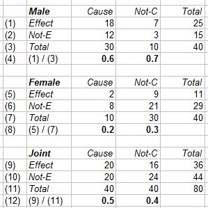
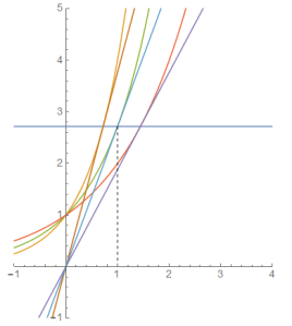
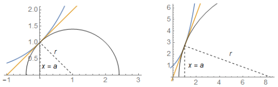
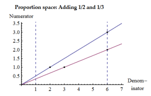
Check also the notion of proportionality in COTP, page 77-78 with the notion of proportion space: {denominator x, numerator y}. Division as a process is a multidimensional notion. The wikipedia article (of today) on proportionality fits this exposition, remarkably with also a diagram of proportion space, with the denominator (cause) on the horizontal axis and the numerator (effect) on the vertical axis (instead of reversed), as it should be because of the difference quotient in calculus. In Conquest of the Plane there is also a vertical line at x = 1, where the numerators give our numbers (a.k.a. slope or tangent).

Conquest of the Plane, p78

Avoiding the word “fraction”

My nomenclature uses the quotient and the distinction in subsets of numbers, and I tend to avoid the word fraction because of apparent confusions that people have. When someone gives a potential confusing definition of fractions, my criticism doesn’t consist of providing a proper definition for fractions, but I point out the confusion, and then refer to the above.

Below, I will also refer to the suggestion by Pierre van Hiele (1973) to abolish fractions (i.e. what people call these), and I will mention a neat trick that provides a much better alternative.

Number means also satisfying a standard form

Number means also satisfying a standard form. Thus “number” is not something mysterious but is a form, like the other forms, yet standardised.

For example, we have 2 / 4 = 1 / 2, yet 1 / 2 has the standard form of the rationals so that 2 / 4 needs to be simplified by eliminating common prime factors. The algebra of 2 / (2 2) = 1 / 2 can be seen as “rewriting the form”.

What the standard is, depends upon the context. We can do sums on natural numbers, integers, rationals, reals. In education students have to learn how to rewrite particular forms into a particular standard. Student need to know the standard forms, not the group theory about the subset of numbers they are working in.

The equality sign in x = a is ambiguous. Computer algebra tends to avoid ambiguity. For example in Mathematica: Set (=) vs Equal (==) vs (identically) SameQ (===). Doing computer algebra would help students to become more precise, compared to current textbooks. Learning is going from vague to precise.

The equality sign in highschool tends to mean “of equal value”, which is above “==”. But two expressions can only be of equal value when they represent the identically same value. Thus x == a would amount to Num[x] === Num[a]. The standard mathematical phrase is “equivalence class” for a number in whichever format, e.g. with the numerical value at the vertical position at line at x = 1 (also for the denominator 1).

The standard form takes one element of an “equivalence class” (depending upon the context of what numbers are on the table, e.g. 1 / 2 for the rationals and 0.5 for the reals). (See COTP p45-48 for issues of “approximation”.)

Multiplication is no procept

Multiplication is no procept. For multiplication there is a clear distinction between the operation 2 * 3 and the resulting number 6. When your teacher asks you to calculate 2 * 3 then the answer of 2 * 3 is correct but likely not accepted. The smart-aleck answer 2 * 3 = 3 * 2 is also correct, but then the context better be group theory.

It is a pity that group theory adopted the name “group theory”. My proposal for elementary school is to replace the complicated word “multiplication” by “group, grouping”. With 12 identical elements, you can make 4 groups of 3. (With identical elements this isn’t combinatorics.) See A child wants nice and no mean numbers (CWNN) (2015). If this use of “group, grouping” is confusing for group theory, then they better change to something like “generalised arithmetic”.

The hijack of number by group theory

The world originally had the notion of number, like counting fingers or measuring distance, but then group theory hijacked the word, and assigned it with a generalised meaning, whence communication has become complicated. Their use of language might cause the need for the term numerical value. I would like to say that 2 is identically the same number in N, Z, Q and R, but group theorists tend to pedantically assert that the notion of number is relative to the set of axioms. In the Middle Ages, people didn’t know negative numbers, and they couldn’t even think about -2. Only by defining -2 as a number too, it could be included as a number. This sounds like Baron von Muenchhausen lifting himself from the swamp. The answer to this is rather that -2 is still a number even though it wasn’t recognised as this. I would like to insist that we use the term “number” for the numerical value in R, so that we can use the word “number” in elementary school in this safe sense. Group theorists then must invent a word of their own, e.g. “generalised number” or “gnumber”, for their systems.

Changing the meaning of words is like that your car is stolen, given another colour, and parked in front of your house as if it isn’t your car. Group theorists tend to focus on group theory. They tend not to look at didactics and teaching. When group theorists hear teachers speaking about numbers, and how 2 is the same number in N and R, then group theorists might smile arrogantly, for they “know better” that N and R are different number systems. This would be misplaced behaviour, for it are the group theorists themselves who hijacked the notion of number and changed its meaning. When research mathematicians have the idea that teachers of mathematics have no training about group theory, then they better read Richard Skemp (1971, 1975), The psychology of learning mathematics, first. This was written with an eye on teaching mathematics (and training teachers) and contains an extensive discussion of group theory. (Though I don’t need to agree with all that Skemp writes.)

Quote on human folly

Peter van ‘t Riet edited Vredenduin (1991) “De geschiedenis van positief en negatief“, Wolters-Noordhoff, on the history of positive and negative numbers. Van ‘t Riet allows himself a concluding observation:

“Kijken wij er achteraf op terug, dan kan een gevoel van verwondering opkomen, dat begrippen die ons zo vanzelfsprekend en helder lijken, zo’n lange ontwikkelingsgeschiedenis hebben gehad waarin vooruitgang, terugval en nieuwe vooruitgang elkaar afwisselden. Opmerkelijk is dat begrippen zich soms pas echt ontwikkelen als zij bevrijd worden van een dominerende idee die eeuwenlang hun ontwikkeling in de weg stond. Dat is bij de negatieve getallen het geval geweest met de geometrisering van de algebra: de gedachte dat getallen representanten waren van meetkundige grootheden is eeuwen achtereen een obstakel geweest teneinde tot een helder begrip van negatieve getallen te komen. Achteraf vraag men zich af: hoe was het mogelijk dat eeuwenlang deze idee de algebra bleef domineren?” (p121)

Since we sometimes check Google Translate for the fun ways of its expressions, it is nice to let the machine speak again:

“If we look afterwards back, then bring up a sense of wonder that concepts which seem to us so obvious and clear, have had such a long history in which progress, relapse and further progress alternating. Remarkably concepts sometimes only really develop as they freed from a dominant idea that for centuries had their development path that is in the negative numbers was the case with the geometrization of algebra:. the idea that numbers representatives were of geometric quantities is centuries successively been an obstacle in order to achieve a clear understanding of negative numbers retrospect one question himself:. how was it possible that for centuries the idea continued to dominate the algebra?” (Google Translate)

Just to be sure: analytic geometry has the number line with negative numbers too. Van ‘t Riet means the line section, that always has a nonnegative length.

A step to answering his question is that mathematicians focus on abstraction, whence they are more guided by their own concepts rather than by empirical applications or the observations in didactics. I included this quote in the hope that group theorists reading this will again grow aware of human folly, and realise that they should support empirical didactics and not block it.

More sources for confusion on formats

More noise is generated by the different “number formats” that have been developed over the course of history. We have forms 2 + ½ = 2½ = 5 / 2 = 25 / 10 = 2.5 = 2 + 2^-1 (neglecting the Egyptians and such). We should not forget that the decimals are actually also a form or result of division. Another example is 0.365 = 3 / 10 + 6 / 100 + 5 / 1000. Only the infinite decimals present a problem, since then we need an infinite series of divisions, yet this can be solved. The various formats have their uses, and thus education must teach students what these are.

An approach might be to only use numbers in decimal notation. However, the expression 1 / 3 is often easier than 0.33333…. Students must learn algebra. Compare 1 / 2 + 1 / 3 with 1 / a + 1 / b.

“But to understand algebra without ever really understood arithmetic is an impossibility, for much of the algebra we learn at school is a generalized arithmetic. Since many pupils learn to do the manipulations of arithmetic with a very imperfect understanding of the underlying principles, it is small wonder that mathematics remain a closed book to them.” (Skemp, p35)

The KNAW 2009 study on arithmetic education and its evidence and research is invalid. It forgot that pupils in elementary school have to learn particular algorithms in arithmetic in preparation for algebra in secondary education. It scored answers to sums as true / false and didn’t assign points to the intermediate steps, so that pupils who used trial and error also had the option to score well. In a 2011 thesis on the psychometrics of arithmetic, the word “algebra” isn’t mentioned, and various of its research results are invalid. There is a rather big Dutch drama on failure of education on arithmetic, failure of supervision, and breaches of integrity of science.

Irrational numbers started as a ratio. Consider a triangle with perpendicular sides 1 and then consider the ratio of the hypothenuse to one of those sides. The input √2 : 1 reduces to number √2.

Standard form for the rationals

There are students who do 2 + ½ = 2½ = 2 ½ = 1, because in handwriting there might appear to be a space that indicates multiplication, compare 2a or 2√2 or 2 km where such a space can be inserted without problem. See the earlier weblog text how Jan van de Craats tortures students. A proposal of mine since 2008 is to use 2 + ½ and stop using 2½.

Yesterday I discovered Poisard & Barton (2007) who compare the teaching of fractions in France and New Zealand, and who also advise 2 + ½. The German wikipedia has also a comment on the confusing notation of 2½. I haven’t looked at the thesis by Rollnik yet.

For a standard form for the rationals, the rules are targeted at facilitating the location on the number line, while we distinguish the operation minus from the sign of a negative number (as -2 = negative 2).

1. If a rational number is equal to an integer, it is written as this integer, and otherwise:
2. The rational number is written as an integer plus or minus a quotient of natural numbers.
3. The integer part is not written when it is 0, unless the quotient part is 0 too (and then the whole is the integer 0).
4. The quotient part has a denominator that isn’t 0 or 1.
5. The quotient part is not written when the numerator is 0 (and then the whole is an integer).
6. The quotient part consists of a quotient (form) with an (absolute) value smaller than 1.
7. The quotient part is simplified by elimination of common primes.
8. When the integer part is 0 then plus is not written and minus is transformed into the negative sign written before the quotient part.
9. When the integer part is nonzero then there is plus or minus for the quotient part in the same direction as the sign of the integer part (reasoning in the same direction).

Thus (- 2 – ½) = (-3 + ½) but only the first is the standard form.

PM 1. Mathematica has the standard form 5 / 2. Conquest of the Plane p54 provides the routine RationalHold[expr] that puts all Rational[x, y] in expr into HoldForm[IntegerPart[expr] + FractionalPart[expr]].

PM 2. Digits are combined into numbers, so that we don’t have 28 = 2 * 8 = 16 = 6. Nice is:

“For example, 7 (4 + a) is equal to 28 + 7a and no 74 + 7a.” (Skemp, p230)

H = -1

A new suggestion is to use H = -1. Then we get 2 + ½ = 2 + 2^H= 5 2^H. Pierre van Hiele (1973) suggested to abolish fractions as we know them. He observed that y / x is a tedious notation, and students have to learn powers anyhow. I agree that the notation y / x generates so-called “mathematics” which is no real mathematics but only is forced by the notation. Using the power of -1 can be confusing because students might think of subtraction, but the use of (abstract) H for the inverse clinches it. See here and my sheets for a workshop of NVvW November 2016.

Above quotient form then becomes (y x^H) and the dynamic quotient (y x^D), in which the brackets may be required in the dynamic case to indicate the scope of the simplification process.

There are students who struggle with a – (-b) = a – (-1) b, perhaps because subtraction actually is a form of multiplication. Curiously, this is another issue of inversion that is made easier by using H, with a – (-b) = a – H b = a + H H b = a + b. See the last weblog entry that division is repeated subtraction. The only requirement is that each number has also an inverse, zero excluded, so that these inverses can be subtracted too. For example 4 3^H = (3 + 1) 3^H = 1 + 3^H translates as repeated subtraction (not for the classroom but for reasons of current exposition):

4 – (1 + 3^H) – (1 + 3^H) – (1 + 3^H) = 4 – 3 (1 + 3^H) = 4 – 3 – 3 3^H = 4 – 3 – 1 = 0

Group theory is for numbers. It is not for education on number formats

The last weblog entry on group theory showed that group theory concentrates on numbers, whence it (cowardly) avoids the perils of education on the various number formats.

Group theory mathematicians will tend to say that 1 / 2 = 2 / 4 = 50 / 100 = .. .are all member of the same “equivalence class” of the number 1 / 2, whence their formats are no longer interesting and can be neglected.

In itself it is a laudable achievement that mathematics has developed a framework that starts with the natural numbers, extends with negative integers, develops the rationals, and finally creates the reals (and then more dimensions). This construction comes along with algorithms, so that we know what works and what doesn’t work for what kind of number. For example, there are useful prime numbers, that help for simplifying rationals. For example 3 * (1 / 3) = 1 whence 3 * 0.3333… = 0.9999… = 1.000… = 1. (Thus the decimal representation is not quite unique, and this is another reason to keep on using rational formats (when possible).)

When these group theory research mathematicians design a training course for aspiring teachers of mathematics, they tend to put most emphasis on group theory, and forget about the various number formats. This has the consequences:

• Teachers from their training become deficient in knowledge about number formats (e.g. Timothy Gowers’s article), even though those are more relevant to teachers because these are relevant for their students.
• There is also conditioning for a future lack of knowledge. The aspiring teachers are trained on abstraction and they will tend to grow blind on the problems that students have when dealing with the various formats.
• All this supports the delusion:

“We should teach group theory so that the students will have less problems with the algebra w.r.t. the various number formats. (For, they can neglect much algebra, like we do, since most forms are all in the same equivalence classes.)” (No quote)

Bas Edixhoven chairs the delusion

Bas Edixhoven (Leiden) is chair of the executive board of Mastermath, a joint Dutch universities effort for the academic education of mathematicians. They also do remedial teaching for students who want to enroll into the regular training for teacher of mathematics but who have deficiencies in terms of mathematics. Think about a biologist who wants to become a teacher of mathematics. For those students the background in empirical science is important, because didactics is an empirical science too. Such students are an asset to education, and they should not be scared away by treating them as if they want to become research mathematicians. Obviously there are high standards of mathematical competence, but this standard is not the same as for doing research in mathematics.

• The “Foundations” syllabus for remedial teaching 2015 written by Edixhoven indeed looks at group theory with the neglect of number formats. The term “fraction” (Dutch “breuk”) is used without definition, while there is also the expression “fraction form” (Dutch “breukvorm”). I get the impression that Edixhoven uses fraction and fraction format as identical. Perhaps he means the procept ? The fractions are not the rationals since apparently π / 2 has a fractional form too.
• At a KNAW conference in 2014 on the education of arithmetic Edixhoven presented standard group theory, presumably thinking that his audience had never heard about it and hadn’t already decided that its role for non-university education is limited. Edixhoven insulted his audience (including me) by not first studying what didacticians like Skemp had already said before about group theory in education.

I find it quite bizarre that mathematics courses at university for training aspiring teachers would neglect the number formats and treat these (remedial) student-teachers as if they want to become research mathematicians. Obviously I cannot really judge on this since I am no research mathematician so that I don’t know what it takes to become one. I only know that I have a serious dislike of it. Yet, the group theory taught is out of focus for what would be helpful for mathematics for teaching mathematics.

PM 1. The Edixhoven 2014 approach at KNAW fits Van Hiele (1973) who also suggests to have a bit of group theory in highschool. Yet, there is the drawback of confusion about the power -1 that students might read as subtraction. I would agree on this idea of having some group theory, but with the use of H = -1 and not without it. Let us first introduce the universal constant H = -1, thus also in elementary school where pupils should learn about division, and then proceed with some group theory in junior highschool.

PM 2. Edixhoven wrote this “Foundations” syllabus together with Theo van den Bogaard who wrote his thesis with Edixhoven. Van den Bogaard has only a few years of experience as teacher of mathematics. Van den Bogaard was secretary of a commission cTWO that redesigned mathematics education in Holland, with a curious idea about “mathematical think activities” (MTA). Van den Bogaard has an official position as trainer of teachers of mathematics but failed to see the error by the psychometrians in the KNAW 2009 study on education on arithmetic. I informed him about my comments on cTWO, MTA and KNAW 2009 but he didn’t respond. Now there is the additional issue of this curious “Foundations” syllabus. Four counts down on didactics and still training aspiring teachers.

Letter to Mastermath

These and other considerations caused me to write this letter to Mastermath.

The following indicates that research mathematicians can have their own subgroups or individuals who meddle with education. None is qualified for education, and one wonders whether they can keep each other in check.

Research mathematicians are at a distance from didactics

Research mathematicians may develop a passion for education and interfere in education, and then start to invent their own interpretations, and then teach those to elementary schools and their aspiring teachers. These mathematicians are not qualified for primary education and apparently think that elementary school allows loose standards (since they can observe errors indeed). Then we get the blind (research mathematicians) helping the deaf (elementary school teachers), but the blind can also be arrogant, and lead the two of them into the abyss.

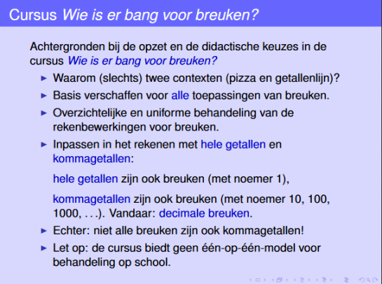
A September 2015 protest concerned Jan van de Craats, now emeritus at UvA. For the topic of division, his name pops up again. In this lecture on fractions for a workshop of 2010 for primary education Van de Craats for example argues as follows (my translation). It is unfair to have criticism on this since these are only sheets. Yet, even sheets should have a consistent set of definitions behind them. These sheets contribute to confusion. Remember that I didn’t give a definition of “fraction”, and that I propose an abolition of what many people apparently call “fraction”.

• Sheet 3: “Three sorts of numbers: integers, decimals, fractions”.
  (a) The main problem is the word “sort”. If he merely means “form” (with the decimals as the standard form that gives “the” number) then this is okay, but if he means that there are really differences (as in group theory) then this is problematic. A professor of mathematics should try to be accurate, and I don’t see why Van de Craats regards “sorts of” as accurate.
  (b) If he identifies fractions with the rationals (but see sheet 26) then we might agree that Z ⊂ Q ⊂ R, though there are group theorists who argue that these are different number systems, and it is not clear whether Van de Craats would ask the group theorists not to meddle in education as he himself is doing.
  (c) My answer: for education it seems best to stick to “various forms, one number (for standard form)”.
• Sheet 30: “A fraction is the outcome of a division.”
  (a) As fraction is a number (Sheet 3), presumable 8 : 4 → 4 / 2 might be acceptable: (i) It is an outcome, (ii) the answer is numerically correct (as it belongs to the equivalence class), (iii) there is no requirement on a standard form (here).
  (b)This doesn’t imply the converse, that the outcome of a division is always a fraction. Then it is either an integer (but then also a fraction (Sheet 25)) or decimal (but then also fraction (Sheet 26)). Thus fraction iff outcome from division.
  (c) PM. My definition was: “Ratio is the input of division. Number is the result of division, if it succeeds.” (COTP p51), which doesn’t define number but distinguishes input and output.
• Sheet 8: “Cito doesn’t test (mixed) fractions anymore in the primary school final examination.” As an observation this might be correct, but if Van de Craats had had proper background in didactics, then he should have been able to spot the error by the psychometricians in the KNAW 2009 report, which should have been sufficient to effect change, instead of setting up this “course in fractions” (that he isn’t qualified for).
• Sheet 18: Pizza model. Didactics shows that students find this difficult. Use a rectangle.
• Sheet 25: “Integers are also fractions (with denominator 1).” On form, students must know the difference between integers and fractions (whatever those might be, see Sheet 30). The answer of (3 – 1) / (2 – 1) = ? better be 2 and not 2 / 1 because the latter can be simplified.
• Sheet 26: “Decimals are also fractions.” Thus fractions are not the rational numbers. The example is that √2 is irrational, also in decimal expansion (a “fraction”). Van de Craats apparently holds fractions and the decimals as identical, only written in different form. Thus also an infinite sum of fractions still is a fraction. A fraction is not just the form of the quotient as defined in Conquest of the Plane and above (though perhaps it can be written like this ?).
• Sheet 27: “However, not all fractions are also decimals.” This is a mystery. There are only three “sorts of” numbers, and w.r.t. Sheet 30 we found that fraction iff division, and all numbers should be divisible by 1. Also, the real numbers contain all numbers we have seen till now (not the complex numbers). Thus there would be phenomena called “fractions” (but still numbers, not algebra) not in the reals ? It cannot be 0 / 0 since the latter would be a result that cannot be accepted. Division 0 : 0 might be a proper question with the answer that the result is undefined. Perhaps he means to say that “1 / 2” doesn’t have the form of “0.5”, and that the expressions differ ? But then we are speaking about form again, and Van de Craats spoke about “sorts of numbers” and not about “same numbers with different forms”.
• Sheet 28: “This course doesn’t offer an one-to-one-model for discussion at school.” It sounds modest but I don’t know what this means. Perhaps he means that the sheets aren’t a textbook.
• Sheet 30: “A fraction is the outcome of a division.”  (I moved this up.)
• Sheet 33: “4 : 7 = 4 / 7”. Apparently the ” : ” stands for the operation of division and “4 / 7” for the result. Apparently Van de Craats wants to get rid of the procept. The equality sign cannot mean identically the same, because otherwise there would be no difference between input and output. Is only 4 / 7 the right answer or is 8 / 14 allowed too ? Perhaps one can teach students that 4 : 7 is a proper question and that 8 / 14 is unacceptable since this must be 4 / 7. However, 4 : 1 would be a proper question too, and then Van de Craats also argues that 4 / 1 would be a fraction (and result of division).
• Sheet 65: “Actually 2 4/5 means 2 + 4/5.” (Van de Craats read an article of mine.) It would have been better if he stated that the first is a horrible convention, and that he proceeded with the second. He calls the form a “mixed fraction” while the English has “mixed number“. Lawyers might have to decide whether “fractions are numbers” implies that a “mixed fraction” is also a “mixed number”.

If a professor of mathematics becomes confused on such an “elementary (school)” issue of fractions (I still don’t know that is meant by this), why would the student believe that anyone can master this apparently superhumanly difficult subject ?

Will the ivory tower stop the blind ?

Would research mathematicians who do group theory be able to correct Van de Craats ?

Let us consider Bas Edixhoven again, see again his sheets.

Or would Edixhoven argue that he himself looks at natural numbers, integers, rationals and reals, so that he has no view on “fractions”, as apparently defined by Van de Craats ? Though the “Foundations” syllabus refers to the word without definition and Edixhoven might presume that aspiring teachers of mathematics know what those fractions are.

Edixhoven in the 2014 lecture only suggests that there better be more proofs and axiomatics in the highschool programme, and he gives the example of a bit of group theory for arithmetic. He also explains  modestly that he speaks “from his own ivory tower” (quote). Thus we can only infer that Edixhoven will remain in this ivory tower and will not stop the blind (but also arrogant) Van de Craats from leading (or at least trying to lead) the deaf (elementary school teachers) into the abyss.

However, professor Edixhoven also left the ivory tower and and joined the real world. At Mastermath he is involved in training aspiring teachers. Since February 2015 he is member of the Scientific Advisory Board of the mathematics department of the University of Amsterdam, where professor Van de Craats still has his homepage with this confusing “course on fractions”. I informed this board in Autumn 2015 about the problematic situation that Van de Craats propounds on primary and secondary education but is not qualified for this. I have seen no correction yet. Apparently Edixhoven doesn’t care or is too busy scaring aspiring teachers away. Apparently, when a teacher of mathematics criticises him, then this teacher obviously must be deficient in mathematics, and should follow a course for due indoctrination in the neglect of didactics of mathematics.

Jan van de Craats, Workshop 2010, page 28