The intuition for the exponential number e

Exponential functions have the form b^x, where b > 0 is the base and x the exponent.

Exponential functions are easily introduced as growth processes. The comparison of x² and 2^x is an eye-opener, with the stories of duckweed or the grain on the chess board. The introduction of the exponential number e is a next step. What intuitions can we use for smooth didactics on e ?

The “discover-e” plot

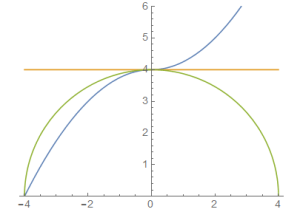
There is the following “intuitive graph” for the exponential number e = 2,71828…. The line y = e is found by requiring that the inclines (tangents) to y = b^x all run through the origin at {0, 0}. The (dashed) value at x = 1 helps to identify the function e^x itself. (Check that the red curve indicates 2^x).

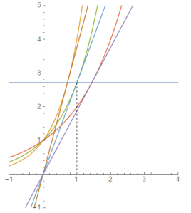
2^x, e^x and 4^x, and inclines through {0, 0}

Remarkably, Michael Range (2016:xxix) also looks at such an outcome e = 2^(1 / c), where c is the derivative of y = 2^x at x = 0, or c = ln[2]. NB. Instead of the opaque term “logarithm” let us use “recovered exponent”, denoted as rex[y].

Perhaps above plot captures a good intuition of the exponential number ? I am not convinced yet but find that it deserves a fair chance.

NB. Dutch mathematics didactician Hessel Pot, in an email to me of April 7 2013, suggested above plot. There appears to be a Wolfram Demonstrations Project item on this too. Their reference is to Helen Skala, “A discover-e,” The College Mathematics Journal, 28(2), 1997 pp. 128–129 (Jstor), and it has been included in the “Calculus Collection” (2010).

Deductions

The point-slope version of the incline (tangent) of function f[x] at x = a is:

y – f[a] = s (x – a)

The function b^x has derivative rex[b] b^x. Thus at arbitrary a:

y – b^a = rex[b] b^a (x – a)

This line runs through the origin {x, y} = {0, 0} iff

0 – b^a = rex[b] b^a (0 – a)

1 = rex[b]  a

Thus with H = -1, a = rex[b]^H = 1 / rex[b]. Then also:

y = f[a] = b^a = b^rex[b]^H = e^(rex[b]  rex[b]^H) = e^1 = e

The inclines running through {0, 0} also run through {rex[b]^H, e}. Alternatively put, inclines can thus run through the origin and then cut y = e .

For example, in above plot, with 2^x as the red curve, rex[2] ≈ 0.70 and a ≈ 1.44, and there we find the intersection with the line y = e.

Subsequently also at a = 1, the point of tangency is {1, e}, and we find with b = e that rex[e] = 1,

The drawback of this exposition is that it presupposes some algebra on e and the recovered exponents. Without this deduction, it is not guaranteed that above plot is correct. It might be a delusion. Yet since the plot is correct, we may present it to students, and it generates a sense of wonder what this special number e is. Thus it still is possible to make the plot and then begin to develop the required math.

Another drawback of this plot is that it compares different exponential functions and doesn’t focus on the key property of e^x, namely that it is its own derivative. A comparison of different exponential functions is useful, yet for what purpose exactly ?

Descartes

Our recent weblog text discussed how Cartesius used Euclid’s criterion of tangency of circle and line to determine inclines to curves. The following plots use this idea for e^x at point x = a, for a = 0 and a = 1.

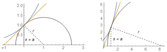
Incline to e^x at x = 0 (left) and x = 1 (right)

Let us now define the number e such that the derivative of e^x is given by e^x itself. At point x = a we have s = e^a. Using the point-slope equation for the incline:

y – f[a] = s (x – a)

y – e^a = e^a (x – a)

y = e^a (x – (a – 1))

Thus the inclines cut the horizontal axis at {x, y} = {a – 1, 0}, and the slope indeed is given by the tangent s = (f[a] – 0) / (a – (a – 1)) = f[a] / 1 = e^a.

The center {u, 0} and radius r of the circle can be found from the formulas of the mentioned weblog entry (or Pythagoras), and check e.g. a = 0:

u = a + s f[a] = a + (e^a)²

r = f[a] √ (1 + s²) = e^a √ (1 + (e^a)²)

A key problem with this approach is that the notion of “derivative” is not defined yet. We might plug in any number, say e^2 = 10 and e^3 = 11. For any location the Pythagorean Theorem allows us to create a circle. The notion of a circle is not essential here (yet). But it is nice to see how Cartesius might have done it, if he had had e = 2.71828….

Conquest of the Plane (COTP) (2011)

Conquest of the Plane (2011:167+), pdf online, has the following approach:

• §12.1.1 has the intuition of the “fixed point” that the derivative of e^x is given by e^x itself. For didactics it is important to have this property firmly established in the minds of the students, since they tend to forget this. This might be achieved perhaps in other ways too, but COTP has opted for the notion of a fixed point. The discussion is “hand waiving” and not intended as a real development of fixed points or theory of function spaces.
• §12.1.2 defines e with some key properties. It holds by definition that the derivative of e^x is given by e^x itself, but there are also some direct implications, like the slope of 1 at x = 0. Observe that COTP handles integral and derivative consistently as interdependent notions. (Shen & Lin (2014) use this approach too.)
• §12.1.3 gives the existence proof. With the mentioned properties, such a number and function appears to exist. This compares e^x with other exponential functions b^x and the recovered exponents rex[y] – i.e. logarithm ln[y].
• §12.1.4 uses the chain rule to find the derivatives of b^x in general. The plot suggested by Hessel Pot above would be a welcome addition to confirm this deduction and extension of the existence proof.
• §12.1.5-7 have some relevant aspects that need not concern us here.
• §12.1.8.1 shows that the definition is consistent with the earlier formal definition of a derivative. Application of that definition doesn’t generate an inconsistency. No limits are required.
• §12.1.8.2 gives the numerical development of e = 2.71828… There is a clear distinction between deduction that such a number exists and the calculation of its value. (The approach with limits might confuse these aspects.)
• §12.1.8.3 shows that also the notion of the dynamic quotient (COTP p57)  is consistent with above approach to e. Thus, the above hasn’t used the dynamic quotient. Using it, we can derive that 1 = {(e^h – 1) // h, set h = 0}. Thus the latter expression cannot be simplified further but we don’t need to do so since we can determine that its value is 1. If we would wish so, we could use this (deduced) property to define e as well (“the formal approach”).

The key difference between COTP and above “approach of Cartesius” is that COTP shows how the (common) numerical development of e can be found. This method relies on the formula of the derivative, which Cartesius didn’t have (or didn’t want to adopt from Fermat).

Difference of COTP and a textbook introduction of e

In my email of March 27 2013 to Hessel Pot I explained how COTP differed from a particular Dutch textbook on the introduction of e.

• The textbook suggests that f ‘[0] = 1 would be an intuitive criterion. This is only partly true.
• It proceeds in reworking f ‘[0] = 1 into a more general formula. (I didn’t mention unstated assumptions in 2013.)
• It eventually boils down to indeed positing that e^x has itself as its derivative, but this definition thus is not explicitly presented as a definition. The clarity of positing this is obscured by the path leading there. Thus, I feel that the approach in COTP is a small but actually key innovation to explicitly define e^x as being equal to its derivative.
• It presents e only with three decimals.

Conclusion

There are more ways to address the intuition for the exponential number, like the growth process or the surface area under 1 / x. Yet the above approaches are more fitting for the algebraic approach. Of these, COTP has a development that is strong and appealing. The plots by Cartesius and Pot are useful and supportive but no alternatives.

The Appendix contains a deduction that was done in the course of writing this weblog entry. It seems useful to include it, but it is not key to above argument.

Appendix. Using the general formula on factor x – a

The earlier weblog entry on Cartesius and Fermat used a circle and generated a “general formula” on a factor x – a. This is not really factoring, since the factor only holds when the curve lies on a circle.

Using the two relations:

f[x] – f[a]  = (x – a)  (2u – x – a) / (f[x] + f[a])    … (* general)

u = a + s f[a]       … (for a tangent to a circle)

we can restate the earlier theorem that s defined in this manner generates the slope that is tangent to a circle. 

f[x] – f[a]  = (x – a)  (2 s f[a] – (x – a)) / (f[x] + f[a]) 

It will be useful to switch to x – a = h:

f[a + h] – f[a]  = h (2 s f[a] – h) / (f[a + h] + f[a]) 

Thus with the definition of the derivative via the dynamic quotient we have:

df / dx = {Δf // Δx, set Δx = 0}

= {(f[a + h] – f[a]) // h, set h = 0}

= { (2 s f[a] – h) / (f[a + h] + f[a]), set h = 0}

= s

This merely shows that the dynamic quotient restates the earlier theorem on the tangency of a line and circle for a curve.

This holds for any function and thus also for the exponential function. Now we have s = e^a by definition. For e^x this gives:

e^{a + h} – e^a  = h (2 s e^a – h) / (e^{a + h} + e^a)

For COTP §12.1.8.3 we get, with Δx = h:

df / dx = {Δf // Δx, set Δx = 0}

= {(e^{a + h} – e^a  ) // h, set h = 0}

= {(2 s e^a – h) / (e^{a + h} + e^a) , set h = 0}

= s

This replaces Δf // Δx by the expression from the general formula, while the general formula was found by assuming a tangent circle, with s as the slope of the incline. There is the tricky aspect that we might choose any value of s as long as it satisfies u = a + s f[a]. However, we can refer to the earlier discussion in §12.1.8.2 on the actual calculation.

The basic conclusion is that this “general formula” enhances the consistency of §12.1.8.3. The deduction however is not needed, since we have §12.1.8.1, but it is useful to see that this new elaboration doesn’t generate an inconsistency. In a way this new elaboration is distractive, since the conclusion that 1 = {(e^h – 1) // h, set h = 0} is much stronger.

Descartes wins from Fermat on the incline

Our protagonists are Cartesius (1596-1650) and Fermat (1607-1665). As Judith Grabiner states, in a recommendable text:

“One could claim that, just as the history of Western philosophy has been viewed as a series of footnotes to Plato, so the past 350 years of mathematics can be viewed as a series of footnotes to Descartes’ Geometry.”  (Grabiner) (But remember Michel Onfray‘s observation that followers of Plato have been destroying texts by opponents. (Dutch readers check here.))

Both Cartesius and Fermat were involved in the early development of calculus. Both worked on the algebraic approach without limits. Cartesius developed the method of normals and Fermat the method of adequality.

Fermat and Δf / Δx

Fermat’s method was algebraic itself, but later has been developed into the method of limits anyhow. When asked what the slope of a ray y = s x is at the point x = 0, then the answer y / x = s runs into problems, since we cannot use 0 / 0. The conventional answer is to use limits. This problem is more striking when one considers the special ray that is defined everywhere except at the origin itself. The crux of the problem lies in the notion of slope Δf / Δx that obviously has a problematic division. With set theory we can now define the “dynamic quotient”, so that we can use Δf // Δx = s even when Δx = 0, so that Fermat’s problem is resolved, and his algebraic approach can be maintained. This originated in 2007, see Conquest of the Plane (2011).

Cartesius and Euclid’s notion of tangency

Cartesius followed Euclid’s notion of tangency. Scholars tend to assign this notion to Cartesius as well, since he embedded the approach within his new idea of analytic geometry.

I thank Roy Smith for this eye-opening question:

“Who first defined a tangent to a circle as a line meeting it only once? From googling, it seems commonly believed that Euclid did this, but it seems nowhere in Euclid does he even state this property of a tangent line explicitly. Rather Euclid gives 4 other equivalent properties, that the line does not cross the circle, that it is perpendicular to the radius, that is a limit of secant lines, and that it makes an angle of zero with the circle, the first of which is his definition, the others being in Proposition III.16. I am wondering where the “meets only once” definition got started. I presume once it got going, and people stopped reading Euclid, (which seems to have occurred over 100 years ago), the currently popular definition took over. Perhaps I should consult Legendre or Hadamard? Thank you for any leads.” (Roy Smith, at StackExchange)

In this notion of tangency there is no problematic division, whence there is no urgency to use limits.

The reasoning is:

• (Circle & Line) A line is tangent to a circle when there is only one common point (or the two intersecting points overlap).
• (Circle & Curve) A smooth curve is tangent to a circle when the  two intersecting points overlap (but the curve might cross the circle at that point so that the notion of “two points” is even more abstract).
• (Curve & Line) A curve is tangent to a line when the above two properties hold (but the line might cross the curve, whence we better speak about incline rather than tangent).

Example of line and circle

Consider the line y = f[x] = c + s x and the point {a, f[a]}. The line can also be written with c = f[a] – s a:

y – f[a] = s (x – a)

The normal has slope –s^H, where we use H = -1. The formula for the normal is the line y – f[a] = –s^H  (x – a). We can choose the center of the circle anywhere on this line. A handy choice is {u, 0}, so that we choose the center on the horizontal axis. (If we looked at a ray and point {0, 0}, then the issue would be similar for {0, c} for nonzero c and thus the approach remains general.) Substituting the point into the normal gives

0 – f[a] = –s^H  (u – a)

s = (u – a) / f[a]

u = a + s f[a]

The circle has the formula (x – u)² + y² = r². Substituting {a, f[a]} generates the value for the radius r² = (a – (a + s f[a]))² + f[a]² = (1 + s²) f[a]² . The following diagram has {c, s, a} = {0, 2, 3} and thus u = 15 and r = 6√5.

 

Method of normals

For the method of normals and arbitrary function f[x], Cartesius’s trick is to substitute y = f[x] into the formula for the circle, and then solve for the unknown center of the circle.

(x – u)² + (y – 0)² = r²

(x – u)² + f[x]² – r² = 0         … (* circle)

This expression is only true for x = a, but we treat it as if it were more general. The key property is:

Since {a, f[a]} satisfies the circle, this equation has a solution for x = a with a double root.

Thus there might be some g such that the root can be isolated:

(x – a)² g [x, u] = 0         … (* roots)

Thus, if we succeed in rewriting the formula for the circle into the form of the formula with the two roots, then we can use information about the structure of the latter to say something about u.

The method works for polynomials, that obviously have roots, but not necessarily for trigonometry and the exponential function.

Algorithm

The algorithm thus is: (1) Substitute f[x] in the formula for the circle. (2) Compare with the expression with the double root. (3) Derive u. (4) Then the line through {a, f[a]} and {u, 0} will give slope –s^H. Thus s = (u – a) / f[a] gives the slope of the incline (tangent) of the curve. (5) If f[a] = 0, add a constant or choose center {u, v}.

Application to the line itself

Consider the line y = f[x] = c + s x again. Let us apply the algorithm. The formula for the circle gives:

(x – u)² + (c + s x)² – r² = 0

x² – 2ux + u² + c² + 2csx + s²x² – r² = 0

(1 + s²) x² – 2 (u – cs) x +  u² + c² – r² = 0

This is a polynomial. It suffices to choose g [x, u] = 1 + s²  so that the coefficients of x² are the same. Also the coefficient of x must be the same. Thus expanding (x – a)²:

(1 + s²) (x² – 2ax +  a²) = 0

– 2 (u – cs)  = -2 a (1 + s²)

u = a (1 + s²) + cs = a + s (c + sa) = a + s f[a]

which is the same result as above.

A general formula with root x – a

We can deduce a general form that may be useful on occasion. When we substitute the point {a, f[a]} into the formula for the circle, then we can find r, and actually eliminate it.

(x – u)² + f[x]² = r² = (a – u)² + f[a]²

f[x]² – f[a]² = (a – u)² – (x – u)²

(f[x] – f[a])  (f[x] + f[a])  = ((a – u) – (x – u))  ((a – u) + (x – u))

(f[x] – f[a])  (f[x] + f[a]) = (a – x)   (a + x – 2u)

f[x] – f[a]  = (a – x)  (a + x – 2u) / (f[x] + f[a])

f[x] – f[a]  = (x – a)  (2u – x – a) / (f[x] + f[a])       … (* general)

f[x] – f[a]  = (x – a) q[x, a, u]

We cannot do much with this, since this is basically only true for x = a and f[x] – f[a] = 0. Yet we have this “branch cut”:

(1)      q[x, a, u] = f[x] – f[a]  / (a – x)        if x ≠ a

(2)      q[a, a, u]      potentially found by other means

If it is possible to “simplify” (1) into another expression Simplify[q[x, a, u]] without the division, then the tantalising question becomes whether we can “simply” substitute x = a. Or, if we were to find q[a, a, u] via other means in (2), whether it links up with (1). These are questions of continuity, and those are traditionally studied by means of limits.

Theorem on the slope

We can still use the general formula to state a theorem.

Theorem. If we can eliminate factors without division, then there is an expression q[x, a, u] such that evaluation at x = a gives the slope s of the line, or q[a, a, u] = s, such that at this point both curve and line are touching the same circle.

Proof. Eliminating factors without division in above general formula gives:

q[x, a, u] =  (2u – x – a) / (f[x] + f[a])

Setting x = a gives:

q[a, a, u] = (u – a) / f[a]

And the above s = (u – a) / f[a] implies that q[a, a, u] = s. QED

This theorem gives us the general form of the incline (tangent).

y[x, a, u] = (x – a) q[a, a, u] + f[a]       …  (* incline)

y[x, a, u] = (x – a) (u – a) / f[a] + f[a] 

PM. Dynamic division satisfies the condition “without division” in the theorem. For, the term “division” in the theorem concerns the standard notion of static division.

Corollary. Polynomials as the showcase

Polynomials are the showcase. For polynomials p[x], there is the polynomial remainder theorem:

When a polynomial p[x] is divided by (x – a) then the remainder is p[a].
(Also, x – a is called a “divisor” of the polynomial if and only if p[a] = 0.)

Using this property we now have a dedicated proof for the particular case of polynomials.

Corollary. For polynomials q[a] = s, with no need for u.

Proof. Now, p[x] – p[a] = 0 implies that x – a is a root, and then there is a “quotient” polynomial q[x] such that:

p[x] – p[a] = (x – a) q[x]

From the general theorem we also have:

p[x] – p[a]  = (x – a) q[x, a, u]

Eliminating the common factor (x – a) without division and then setting x = a gives q[a] = q[a, a, u] = s. QED

We now have a sound explanation why this polynomial property gives us the slope of the polynomial at that point. The slope is given by the incline (tangent), and it must also be slope of the polynomial because of the mutual touching of the same circle.

See the earlier discussion about techniques to eliminate factors of polynomials without division. We have seen a new technique here: comparing the coefficients of factors.

Second corollary

Since q[x] is a polynomial too, we can apply the polynomial remainder theorem again, and thus we have q[x] = (x – a) w[x] + q[a] for some w[x]. Thus we can write:

p[x] = (x – a) q[x] + p[a] 

p[x] = (x – a) ( (x – a) w[x] + q[a] ) + p[a]       … (* Ruffini’s Rule twice)

p[x] = (x – a)² w[x] + (x – a) q[a] + p[a]           … (* Range’s proof)

p[x] = (x – a)² w[x] + y[x, a]                             … (* with incline)

We see two properties:

• The repeated application of Ruffini’s Rule uses the indicated relation to find both s = q[a] and constant f[a], as we have seen in last discussion.
• Evaluating f[x] / (x – a)² gives the remainder y[x, a], which is the formula for the incline.

Range’s proof method

Michael Range proves q[a] = s as follows (in this article (p406) or book (p32)). Take above (*) and determine the error by substracting the line y = s (x – a) + p[a] :

error = p[x] – y = (x – a)² w[x] + (x – a) q[a] – s (x – a)

= (x – a)² w[x] + (x – a) (q[a] – s)

The error = 0 has a root x = a with multiplicity greater than one if and only if s = q[a].

Direct application to the incline itself

Now that we have established this theory, there may be no need to refer to the circle explicitly. It can suffice to use the property of the double root. Michael Range (2014) gives the example of the incline (tangent) at x² at {a, a²}. The formula for the incline is:

f[x] – f[a]  = s (x – a)

x² – a² – s (x – a) = 0

 (x – a) (x + a – s) = 0

There is only a double root or (x – a)² when s = 2a.

Working directly on the line allows us to focus on s, and we don’t need to determine q[x] and plug in x = a.

Michael Range (2011) clarifies – with thanks to a referee – that the “point-slope” form of a line was introduced by Gaspard Monge (1746-1818), and that Descartes apparently did not think about this himself and thus neither to plug in y = f [x] here. However, observe that we only can maintain that there must be a double root on this line form too, since {a, f[a]} still lies on a tangent circle.

[Addendum 2017-01-10: The later argument in a subsequent weblog entry becomes: If the function can be factored twice, then there is no need to refer to the circle. But when this would be equivalent to the circle then such a distinction is immaterial.]

Addendum. Example of function crossing a circle

When a circle touches a curve, it still remains possible that the curve crosses the circle. The original idea of two points merging together into an overlapping point then doesn’t apply anymore, since there is only one intersecting point on either side if the circle were smaller or bigger.

An example is the spline function g[x] = {If x < 0 then 4 – x² / 4 else 4 + x² / 4}. This function is C1 continuous at 0, meaning that the sections meet and that the slopes of the two sections are equal at 0, while the second and higher derivatives differ. The circle with center at {0, 0} and radius 4 still fits the point {0, 4}, and the incline is the line y = 4.

An application of above algorithm would look at the sections separately and paste the results together. Thus this might not be the most useful example of crossing.

In this example there might be no clear two “overlapping” points. However, observe:

• Lines through {0, 4} might have three points with the curve, so that the incline might be seen as having three overlapping points.
• Points on the circle can always be seen as the double root solutions for tangency at that point.

Addendum. Discussion

There is still quite a conceptual distance between (i) the story about the two overlapping points on the circle and (ii) the condition of double roots in the error between line and polynomial.

The proof given by Range uses the double root to infer the slope of the incline. This is mathematically fine, but this deduction doesn’t contain a direct concept that identifies q[a] as the slope of an incline (tangent): it might be any line.

We see this distinction between concept and algorithm also in the direct application to Monge’s point-slope formulation of the line. Requiring a double root works, but we can only do so because we know about the theory about the tangent circle.

The combination of circle and line remains the fundamental reason why there are two roots. Thus the more general proof given above, that reasons from the circle and unpacks f[x]² – f[a]² into the conditions for incline and its normal, is conceptually more attractive. I am new to this topic and don’t know whether there are references for this general proof.

Conclusions

(1) We now understand where the double root comes from. See the earlier discussion on polynomials, Ruffini’s rule and the meaning of division (see the section on “method 2”).

(2) There, we referred to polynomial division, with the comment: “Remarkably, the method presumes x ≠ a, and still derives q[a]. I cannot avoid the impression that this method still has a conceptual hole.” However, we now observe that we can compare the values of the coefficients of the powers of x, whence we can avoid also polynomial division.

(3) There, we had a problem that developing p[x] = (x – a)² w[x] + y[x, a] didn’t have a notion of tangency, in terms of Δf / Δx. However, we actually have a much older definition of tangency.

(4) The above states an algorithm and a general theorem with the requirements that must be satisfied.

(5) Cartesius wins from Fermat on this issue of the incline (tangent), and actually also on providing an exact method for polynomials, where Fermat introduced the problem of error.

(6) For trigonometry and exponentials we know that these can be written as power series, and thus the Cartesian method would also apply. However, the power series are based upon derivatives, and this would introduce circularity. However, the method of the dynamic quotient from 2007 still allows an algebraic result. The further development from Fermat into the approach with limits would become relevant for more complex functions.

PM. The earlier discussion referred to Peter Harremoës (2016) and John Suzuki (2005) on this approach. New to me (and the book unread) are: Michael Range (2011), the recommendable Notices, or the book (2015) – review Ruane (2016) – and Shen & Lin (2014).

Cartesius, Portrait by Frans Hals 1648